
Spherical cows & NeurIPS 2025
I guess in my heart I am still a physicist: When I learn about a simplified toy-model (a spherical cow) explanation that captures the essence of a complex phenomenon, I feel elated. I had this experience multiple times in NeurIPS this year, and I’d like to share the respective papers with you. Let’s dive right in.

Scaling laws derived
Superposition Yields Robust Neural Scaling by Y. Liu et al. (best paper)
The last few years were, as Ilya Sutzkever said, the years of scaling, fueled by the belief that model performance will scale with data size, compute size and model size. Some specific empirical relationships between model performance and the various scale factors became known as the “scaling laws”. Dario Amodei admits that this is a misnomer, because there’s no known law or theorem that mandates them.
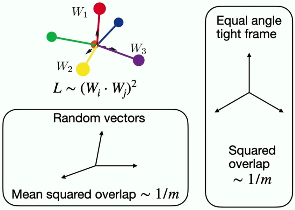
That’s why I loved the paper above. They show using a toy model that a power law scaling of the loss with model size (at least the representation size) follows from the need to embed a large number of concepts in a smaller-dimensional space. They show that the scaling law established using this spherical cow model holds empirically on published LLMs.
Why diffusion models generalize?
On the Closed-Form of Flow Matching: Generalization Does Not Arise from Target Stochasticity, by Q. Bertrand et al.
Why Diffusion Models Don’t Memorize: The Role of Implicit Dynamical Regularization in Training, by T. Bonnaire et al. (best paper)
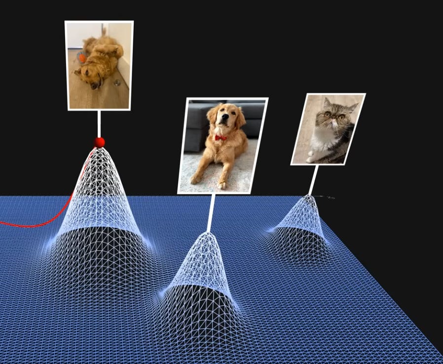
Diffusion models are a means to sample from the distribution of natural images. As Julia Turc’s video explains, the images the model was trained on serve like spikes in that distribution of images, and diffusion is the “blurring” and then the progressive “deblurring” of these spikes, which helps finding them starting from noise (because it’s easier to find a blurred spike than an infinitely thin one).
But why, then, do diffusion models generalize, rather than snapping each input image to the closest one in the training data? Per the presenters of the papers above, this is an unanswered question, which they try to tackle. Both do it beautifully, IMO.
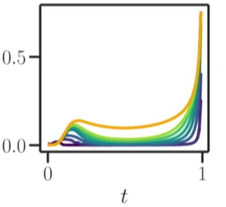
The first paper does this by comparing diffusion performed by a denoising deep network to the diffusion that we’d obtain with a closed-form denoising based on the training data. Yep, given a training dataset, denoising has a closed non-parametric form! Inefficient to calculate, but closed. The closed form inevitably drives towards one of the images in the training set. So where does the approximation by a network deviate from that fate?
As the figure below shows, in two points in time: Towards the beginning of the denoising, and towards the end. To me it’s still a mystery why this happens, and why this happens in a way that results in, of all things, photorealistic images. But the paper beautifully visualizes when this deviation happens.
The second paper addresses the phenomenon illustrated in the image below: the area marked as “Dynamical Regularization” is the area where the network has enough capacity to overfit to the closed form solution, and yet it doesn’t. Why?
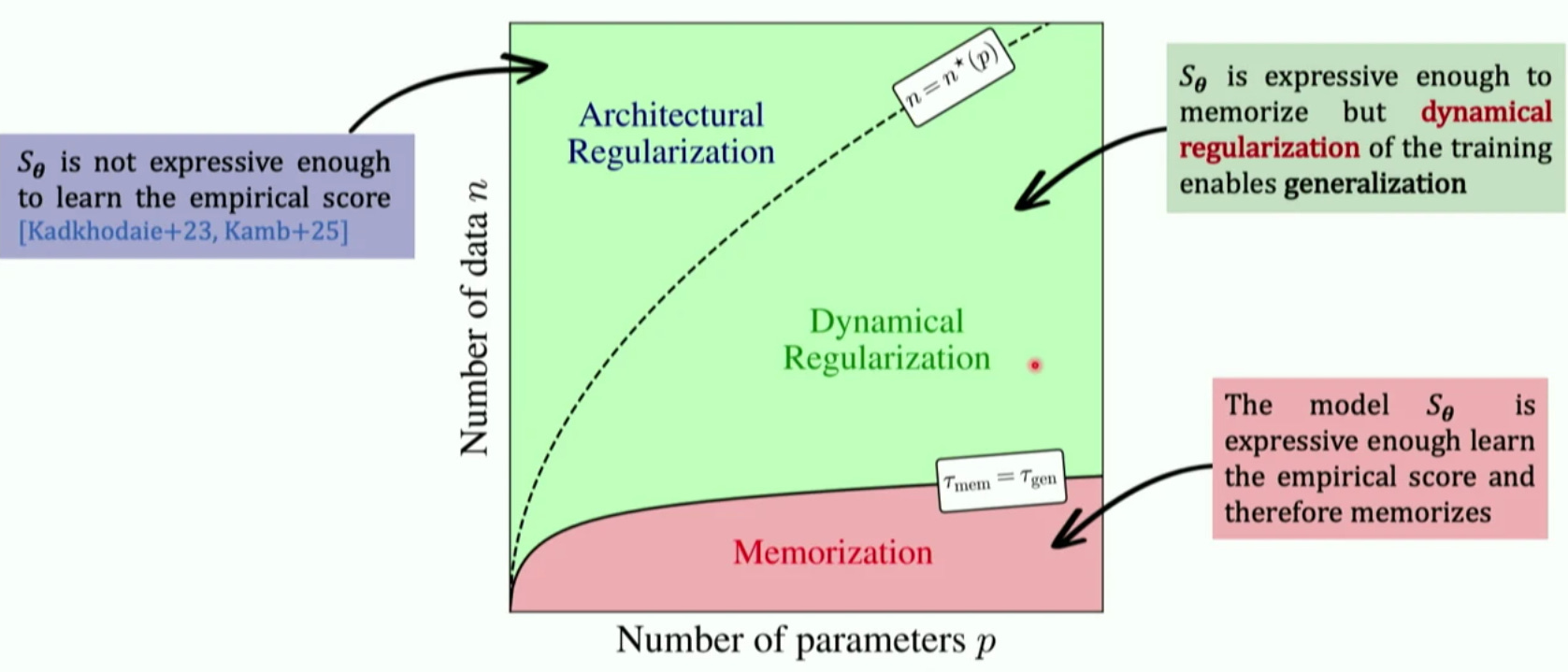
Their explanation is a spherical cow model. They study the eigenvalues of the flow induced by a simple diffusion model, and find that dynamics that is related to overfiting is associated with smaller (slower) eigenvalues than dynamics associated with generalization. In other words, diffusion networks generalize because their training dynamics prioritizes learning the structure before the memorizing. That’s why early stopping works. I guess there may have been prior work on the mechanics of early stopping, but this is the first time I saw such a lucid explanation.
Neural activity in rodents explained by a low-dimensional activation space
High-dimensional neuronal activity from low-dimensional latent dynamics: a solvable model by V. Schmutz et al.
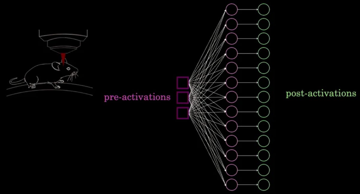
The neuron-firing pattern in the visual cortex of mice is high-dimensional: The PCA analysis of 1000 neurons has a power-law decay of the eigenvalues, which means that there’s no clear cutoff below which dimensions are “unimportant”. However the paper shows that if we assume a latent vector dimension of N, on which we apply an MLP that maps it to the full 1000 dimensions and activates the result, the latent vector’s PCA has a very few non-negligible eigenvalues: N=7 when the mice are not looking at anything, and N=94 when they are. And guess what - it turns out that the state in this low-dimensional space correlates well with the state of the animal.
Read the paper to see how they did it - it’s a very neat and simple method. And as a bonus, there’s also a spherical cow: an exactly-solvable network where a 2 dimensional pre-activation space gives rise to a full-dimensional post-activation space.
Are two transformers trained in the same way equivalent in some way?
Generalized Linear Mode Connectivity for Transformers by A. Theus et al.
Per their presentation, prior work showed that when two identical MLPs or CNNs are trained in the same way (but with different initializations and other randomness related to training), the models will be “the same” in the following sense: Up to a permutation of the neurons, we can linearly interpolate between the weights of the two models and the loss will stay the same throughout the interpolation.
This makes sense: Once we got the permutation out of the way, we’re left with a “valley of degeneracy” or an “affine subspace” where the loss stays the same. Different instances of the model will thus land in different points in this affine subspace. Put simply, the weights of the models will be the same up to a permutation + a translation in the affine subspace.
The point the paper makes is that with transformers, there are parts of the computation where there’s no activation, and because of that, instead of just a permutation invariance, we have invariance to a linear transformation, or, since we’re layer-normalizing, invariance up to an orthogonal transformation. Put simply, in transformers, two models will be related by an orthogonal transformation + a translation in the affine subspace (except for the parts that have activation, where it’s still permutation + a translation in the affine subspace).
The paper shows how to overcome this broader invariance, but my main takeaway is not the method but the relation to the the next section: The residual streams of two transformers that were trained in the same way will be the same up to an orthogonal transformation. This is profound. Angles between embedding vectors (and lengths thereof) are preserved. Am I connecting the dots correctly? Correct me if I misunderstood 🙂.
Bonus (not from NeurIPS): Transformers explained
A Mathematical Framework for Transformer Circuits by N Elhage et al (Dec 2021).
This is not from NeurIPS, but I loved it so much, and it relates so well to spherical cows, that I wanted to include it here.
I was always uncomfortable with the common explanation of transformers - namely that it’s similar to a document retrieval problem and hence has keys and values. I appreciate that the document-retrieval analogy led the authors to the idea, but something as important and as general as a Transformer ought to be explainable in more than one way, or so I felt.
There are many great resources on transformers (I link some at the end), but here’s what I loved about the one above:
The explanation transcends keys and values and queries and deems them superficial. The attention weight between token i and token j looks like a dot product between the respective vectors with a matrix in between, and this matrix is made low rank by factoring it to a Query matrix times a Key matrix. Similarly, the (Output matrix) × (Value matrix) is also a low-rank factorization of the matrix that, loosely speaking, transitions an embedding vector to the next layer. I’ll stop butchering their explanation here - go read it 🙂.
Their toy examples of what a zero-layer, one-layer and two-layer transformers do is extremely enlightening and demystifying.
Their description of how information flows through the residual stream is simple, clear and offers multiple powerful insights (for example, there’s that the residual stream has no privileged basis - see the orthogonal transformation thing above).
I felt like I’m reading a very clearly written textbook, which goes above and beyond in its attempts to explain and elucidate.
Of course, there are some other great resources, especially videos: